value that appears most often in a set of data
Videos
Saying "the mode" implies that the distribution has one and only one. In general a distribution may have many modes, or (arguably) none.
If there's more than one mode you need to specify if you want all of them or just the global mode (if there is exactly one).
Assuming we restrict ourselves to unimodal distributions*, so we can speak of "the" mode, they're found in the same way as finding maxima of functions more generally.
*note that page says "as the term "mode" has multiple meanings, so does the term "unimodal"" and offers several definitions of mode -- which can change what, exactly, counts as a mode, whether there is 0 1 or more -- and also alters the strategy for identifying them. Note particularly how general the "more general" phrasing of what unimodality is in the opening paragraph "unimodality means there is only a single highest value, somehow defined"
One definition offered on that page is:
A mode of a continuous probability distribution is a value at which the probability density function (pdf) attains its maximum value
So given a specific definition of the mode you find it as you would find that particular definition of "highest value" when dealing with functions more generally, (assuming that the distribution is unimodal under that definition).
There are a variety of strategies in mathematics for identifying such things, depending on circumstances. See, the "Finding functional maxima and minima" section of the Wikipedia page on Maxima and minima which gives a brief discussion.
For example, if things are sufficiently nice -- say we're dealing with a continuous random variable, where the density function has continuous first derivative -- you might proceed by trying to find where the derivative of the density function is zero, and checking which type of critical point it is (maximum, minimum, horizontal point of inflexion). If there's exactly one such point which is a local maximum, it should be the mode of a unimodal distribution.
However, in general things are more complicated (e.g. the mode may not be a critical point), and the broader strategies for finding maxima of functions come in.
Sometimes, finding where derivatives are zero algebraically may be difficult or at least cumbersome, but it may still be possible to identify maxima in other ways. For example, it may be that one might invoke symmetry considerations in identifying the mode of a unimodal distribution. Or one might invoke some form of numerical algorithm on a computer, to find a mode numerically.
Here are some cases that illustrate typical things that you need to check for - even when the function is unimodal and at least piecewise continuous.
So, for example, we must check endpoints (center diagram), points where the derivative changes sign (but may not be zero; first diagram), and points of discontinuity (third diagram).
In some cases, things may not be so neat as these three; you have to try to understand the characteristics of the particular function you're dealing with.
I haven't touched on the multivariate case, where even when functions are quite "nice", just finding local maxima may be substantially more complex (e.g. the numerical methods for doing so can fail in a practical sense, even when they logically must succeed eventually).
This answer focuses entirely on mode estimation from a sample, with emphasis on one particular method. If there is any strong sense in which you already know the density, analytically or numerically, then the preferred answer is, in brief, to look for the single maximum or multiple maxima directly, as in the answer from @Glen_b.
"Half-sample modes" may be calculated using recursive selection of the half-sample with the shortest length. Although it has longer roots, an excellent presentation of this idea was given by Bickel and Frühwirth (2006).
The idea of estimating the mode as the midpoint of the shortest interval that contains a fixed number of observations goes back at least to Dalenius (1965). See also Robertson and Cryer (1974), Bickel (2002) and Bickel and Frühwirth (2006) on other estimators of the mode.
The order statistics of a sample of  values of
  are defined by
  .
.
The half-sample mode is here defined using two rules.
Rule 1. If  , the half-sample mode is
  . If
. If  , the half-sample mode is
  . If
. If  , the half-sample mode is
  if
if  and
and  are closer than
  and
and  ,
,  if
the opposite is true, and
if
the opposite is true, and  otherwise.
Rule 2. If  , we apply recursive selection until left with
  or fewer
values. First let
or fewer
values. First let  . The shortest half of the data from rank
  to rank
  is identified to minimise
  over
over  . Then the shortest half of those
  values is identified using
  , and so on. To finish, use Rule 1.
The idea of identifying the shortest half is applied in the "shorth" named
by J.W. Tukey and introduced in the Princeton robustness study of
estimators of location by Andrews, Bickel, Hampel, Huber, Rogers and Tukey
(1972, p.26) as the mean of the shortest half-length  for
for  . Rousseeuw (1984), building on a suggestion by Hampel (1975), pointed out that the midpoint of the shortest half
  is the least median of squares (LMS) estimator of location for
  . See Rousseeuw (1984) and Rousseeuw and Leroy (1987) for
applications of LMS and related ideas to regression and other problems.
Note that this LMS midpoint is also called the shorth in some more recent
literature (e.g. Maronna, Martin and Yohai 2006, p.48). Further, the
shortest half itself is also sometimes called the shorth, as the title of
Grübel (1988) indicates. For a Stata implementation and more detail, see
. See Rousseeuw (1984) and Rousseeuw and Leroy (1987) for
applications of LMS and related ideas to regression and other problems.
Note that this LMS midpoint is also called the shorth in some more recent
literature (e.g. Maronna, Martin and Yohai 2006, p.48). Further, the
shortest half itself is also sometimes called the shorth, as the title of
Grübel (1988) indicates. For a Stata implementation and more detail, see
shorth from SSC.
Some broad-brush comments follow on advantages and disadvantages of half-sample modes, from the standpoint of practical data analysts as much as mathematical or theoretical statisticians. Whatever the project, it will always be wise to compare results with standard summary measures (e.g. medians or means, including geometric and harmonic means) and to relate results to graphs of distributions. Moreover, if your interest is in the existence or extent of bimodality or multimodality, it will be best to look directly at suitably smoothed estimates of the density function.
Mode estimation By summarizing where the data are densest, the half-sample mode adds an automated estimator of the mode to the toolbox. More traditional estimates of the mode based on identifying peaks on histograms or even kernel density plots are sensitive to decisions about bin origin or width or kernel type and kernel half-width and more difficult to automate in any case. When applied to distributions that are unimodal and approximately symmetric, the half-sample mode will be close to the mean and median, but more resistant than the mean to outliers in either tail. When applied to distributions that are unimodal and asymmetric, the half-sample mode will typically be much nearer the mode identified by other methods than either the mean or the median.
Simplicity The idea of the half-sample mode is fairly simple and easy to explain to students and researchers who do not regard themselves as statistical specialists.
Graphic interpretation The half-sample mode can easily be related to standard displays of distributions such as kernel density plots, cumulative distribution and quantile plots, histograms and stem-and-leaf plots.
At the same time, note that
Not useful for all distributions When applied to distributions that are approximately J-shaped, the half-sample mode will approximate the minimum of the data. When applied to distributions that are approximately U-shaped, the half-sample mode will be within whichever half of the distribution happens to have higher average density. Neither behaviour seems especially interesting or useful, but equally there is little call for single mode-like summaries for J-shaped or U-shaped distributions. For U shapes, bimodality makes the idea of a single mode moot, if not invalid.
Ties The shortest half may not be uniquely defined. Even with measured data, rounding of reported values may frequently give rise to ties. What to do with two or more shortest halves has been little discussed in the literature. Note that tied halves may either overlap or be disjoint.
The procedure adopted in the Stata implementation hsmode given  ties is to use the middlemost in order, except that that is in turn not uniquely defined unless
  is
odd. The middlemost is arbitrarily taken to have position
is
odd. The middlemost is arbitrarily taken to have position  in order, counting upwards. This is thus the 1st of 2, the 2nd of 3 or 4, and so forth.
This tie-break rule has some quirky consequences. Thus with values  , the rules yield
  as the half-sample mode, not
  as
would be natural on all other grounds. Otherwise put, this problem can
arise because for a window to be placed symmetrically the window length
as
would be natural on all other grounds. Otherwise put, this problem can
arise because for a window to be placed symmetrically the window length
 must be odd for odd
  and even for even
  , which is
difficult to achieve given other desiderata, notably that window length
should never decrease with sample size. We prefer to believe that this
is a minor problem with datasets of reasonable size.
, which is
difficult to achieve given other desiderata, notably that window length
should never decrease with sample size. We prefer to believe that this
is a minor problem with datasets of reasonable size.
Rationale for window length Why half is taken to mean  also does not appear to be discussed. Evidently we need a rule that yields
a window length for both odd and even
also does not appear to be discussed. Evidently we need a rule that yields
a window length for both odd and even  ; it is preferable that the rule be
simple; and there is usually some slight arbitrariness in choosing a rule
of this kind. It is also important that any rule behave reasonably for
small
; it is preferable that the rule be
simple; and there is usually some slight arbitrariness in choosing a rule
of this kind. It is also important that any rule behave reasonably for
small  : even if a program is not deliberately invoked for very small
sample sizes the procedure used should make sense for all possible sizes.
Note that, given
: even if a program is not deliberately invoked for very small
sample sizes the procedure used should make sense for all possible sizes.
Note that, given  the half-sample mode is just the single sample
value, and, given
the half-sample mode is just the single sample
value, and, given  , it is the average of the two sample values. A
further detail about this rule is that it always defines a slight majority,
thus enforcing democratic decisions about the data. However, there seems
no strong reason not to use
, it is the average of the two sample values. A
further detail about this rule is that it always defines a slight majority,
thus enforcing democratic decisions about the data. However, there seems
no strong reason not to use  as an even simpler rule, except that if it makes much difference, then it is likely that your sample size
or variable is unsuitable for the purpose.
as an even simpler rule, except that if it makes much difference, then it is likely that your sample size
or variable is unsuitable for the purpose.
Robertson and Cryer (1974, p.1014) reported 35 measurements of uric acid
(in mg/100 ml):  The Stata implementation
 hsmode reports a mode of 5.38. Robertson and Cryer's own estimates using a rather different procedure are  . Compare with your favourite density estimation procedure.
Andrews, D.F., P.J. Bickel, F.R. Hampel, P.J. Huber, W.H. Rogers and J.W. Tukey. 1972. Robust estimates of location: survey and advances. Princeton, NJ: Princeton University Press.
Bickel, D.R. 2002. Robust estimators of the mode and skewness of continuous data. Computational Statistics & Data Analysis 39: 153-163.
Bickel, D.R. and R. Frühwirth. 2006. On a fast, robust estimator of the mode: comparisons to other estimators with applications. Computational Statistics & Data Analysis 50: 3500-3530.
Dalenius, T. 1965. The mode - A neglected statistical parameter. Journal, Royal Statistical Society A 128: 110-117.
Grübel, R. 1988. The length of the shorth. Annals of Statistics 16: 619-628.
Hampel, F.R. 1975. Beyond location parameters: robust concepts and methods. Bulletin, International Statistical Institute 46: 375-382.
Maronna, R.A., R.D. Martin and V.J. Yohai. 2006. Robust statistics: theory and methods. Chichester: John Wiley.
Robertson, T. and J.D. Cryer. 1974. An iterative procedure for estimating the mode. Journal, American Statistical Association 69: 1012-1016.
Rousseeuw, P.J. 1984. Least median of squares regression. Journal, American Statistical Association 79: 871-880.
Rousseeuw, P.J. and A.M. Leroy. 1987. Robust regression and outlier detection. New York: John Wiley.
This account is based on documentation for
Cox, N.J. 2007. HSMODE: Stata module to calculate half-sample modes, http://EconPapers.repec.org/RePEc:boc:bocode:s456818.
See also David R. Bickel's website here for information on implementations in other software.
 is a random variable which takes values in
  then the $mode$ is the value
  for which
  is maximised, in other words the point
  at which the p.m.f.
  is a maximum. There may be many such points, in which case there is more than one $mode$. These points are not necessarily always next to each other.
 at which the density function
  is a maximum. This can usually be found by differentiating the density function to find the points where the derivative is zero and then, importantly, also checking whether such points are actually maxima.