


A simpler approach to this
At the beginning of column B, type
=UNIQUE(A:A)
Then in column C, use
=COUNTIF(A:A, B1)
and copy them in all row column C.
Edit: If that doesn't work for you, try using semicolon instead of comma:
=COUNTIF(A:A; B1)
I have a google sheet that consists of 6 data sheets and 1 summary sheet.
I wanna tally up the amount of times a certain value appears across all 6 data sheets. I’m planning to include this tally in the summary sheet. Anyone have a formula for this?
A simpler approach to this
At the beginning of column B, type
=UNIQUE(A:A)
Then in column C, use
=COUNTIF(A:A, B1)
and copy them in all row column C.
Edit: If that doesn't work for you, try using semicolon instead of comma:
=COUNTIF(A:A; B1)
Try:
=ArrayFormula(QUERY(A:A&{"",""};"select Col1, count(Col2) where Col1 != '' group by Col1 label count(Col2) 'Count'";1))
22/07/2014 Some time in the last month, Sheets has started supporting more flexible concatenation of arrays, using an embedded array. So the solution may be shortened slightly to:
=QUERY({A:A,A:A},"select Col1, count(Col2) where Col1 != '' group by Col1 label count(Col2) 'Count'",1)
google sheets - Count occurences - Web Applications Stack Exchange
Count how many times a value occurs in a range of cells. - Google Docs Editors Community
google sheets - list all unique values and count how many times each appears - Stack Overflow
google sheets - How to count the number of times a unique value appears in a list? - Stack Overflow
Does Coefficient work with both Google Sheets and Excel?
What is Coefficient's AI Sheets Assistant?
How does Coefficient's automated refresh work?
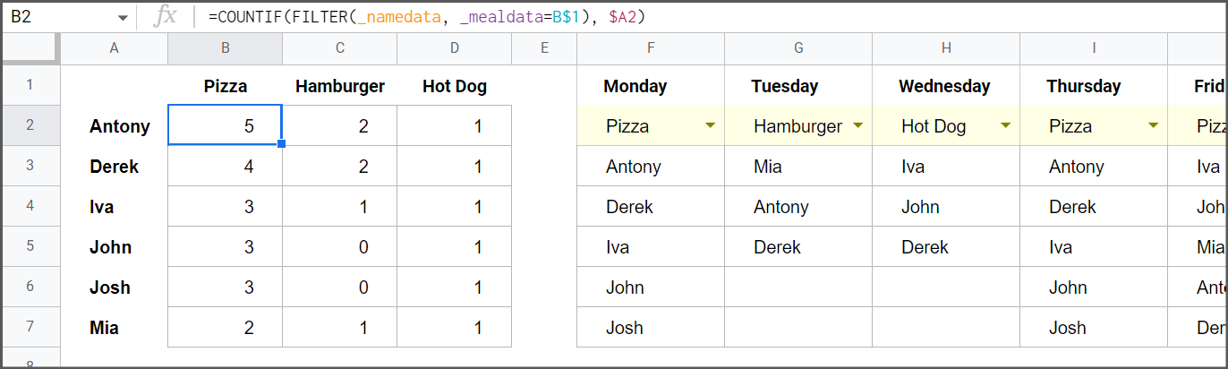
COUNTIF & FILTER
- The COUNTIF function returns a conditional count across a range;
=COUNTIF(range, criterion)
- The FILTER function returns a filtered version of the source range, returning only rows or columns that meet the specified conditions.
=FILTER(range, condition1, [condition2, ...])
- By combining COUNTIF & FILTER one can FILTER the data across all days based on a
menuitem, then use COUNTIF to count occurrences of anamein the filtered data.
Named Ranges in Formulas
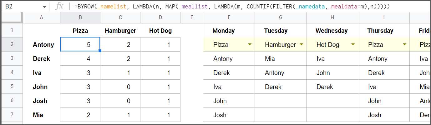
The formula can be adapted for a LAMBDA function
| name | range | note |
|---|---|---|
| _mealdata | F2:O2 |
Daily meals data entries |
| _namedata | F3:O7 |
Daily names data entries |
| _namelist | A2:A7 |
List of names for filtering data |
| _meallist | B1:D1 |
List of meals for filtering data |
First Formula
Formula uses named ranges to make the code easier to manage.
=COUNTIF(FILTER(_namedata, _mealdata=B A2)
A2)
LAMBDA Function
=BYROW(_namelist, LAMBDA(n, MAP(_meallist, LAMBDA(m, COUNTIF(FILTER(_namedata,_mealdata=m),n)))))
I don’t know if this option would be easier, but for me the formula
=SUM(ARRAYFORMULA(IF( 4:
4: 9=
9= E
E J
J 3),0)))
placed in cell B4 and then stretched over the entire range B4:D9 gave the same result as that of our respected colleagues Blind Spots and doubleunary
You can select your whole range in a query like this (change A2:F with your desired range)
=QUERY(FLATTEN(A2:F),"SELECT Col1,COUNT(Col1) where Col1 is not null group by Col1")

See this answer on how to stack unique counts when values are in multiple columns. For example if your data is in A1:D10:
=UNIQUE({A1:A10;B1:B10;C1:C10;D1:D10})
Will return a (vertical) list of all unique values. Then use countif in a new column on the whole range (rows, columns) with condition on each of the unique values.
