Not sure how this is done in the any specific library, but here is what I would try.

Given two sets of points ( points in the first set and in the second set): and , all in -dimensional space ()

I would compute the 'centres of mass' of the two sets:

I would then use the mid-point between the two centres of mass,

as the point for the hyper-plane.

Then I would use the vector connecting the two centres of mass,

as the normal for the hyper-plane. Lets define

A single point and a normal vector, in -dimensional space, will uniquely define an dimensional hyper-plane. To actually do it you will need to find a set of vectors

This set can be created by Gram-Schmidt type process, starting from your trivial basis and then ensuring that every new vector is orthogonal to all vectors in the set and to .

Once you did that, any point on the hyper-plane will be uniquely described by coordinates , and will correspond to the following point in the original -dimensional space

This is an excellent question and one I struggled with as well.

Firstly, the margin is not fixed. As your diagram shows, the margin $m = \frac{2}{\lVert w \rVert}$, which is a function of the 2-norm of the $w$ parameter, nothing else. So the margin is maximized by minimizing the norm of $w$.

But let's back up to see why.

We have some data represented as vectors $x_i \in \mathbb{R}^n$ and each $x_i$ is associated with a binary label $y_i \in \{-1,1\}$, for $i \in \mathbb{N}$. We could have made the labels anything, but choosing -1 and 1 is mathematically convenient.

An (affine) hyperplane is the generalization of a line in n-dimensional space defined as the set of points $x$ such that $w^Tx + b = 0$, where $w, x \in \mathbb{R}^n$ and $w^Tx$ is the dot (inner) product between these vectors. The choice of $w$ will change the orientation of the hyperplane and the choice of $b$ will determine its offset from the origin.

We want to find a hyperplane (i.e. choice of $w, b$) that separates the data $x_i$ according to their class labels. We assume our data can be perfectly separated by a line (or hyperplane), i.e. it is linearly separable. So we want a hyperplane such that when $y_i = -1$ then $w^Tx_i + b \le 0$ and when $y_i = 1$ then $w^Tx_i + b \ge 0$. There's actually a fairly straightforward algorithm called the perceptron algorithm that can find a hyperplane meeting those constraints.

But there are an infinite number of hyperplanes (i.e. choices of $w, b$) that can satisfy the constraints of separating the data classes, so in order for our hyperplane to work well in classifying future data, we want it to optimally separate the data classes such that it is not biased toward one class or another and is situated perfectly between them with maximal space on either side (maximal margins).

The easier way to set this up is that what we really want is to define two parallel hyperplanes, one just on the inside boundary of class $y_i = -1$ and the other just on the inside boundary of the class $y_i = 1$, then the actual decision boundary will be the parallel hyperplane exactly in the middle of these.

In other words, if we have our decision boundary hyperplane as $w^Tx + b = 0$, then we want to find a $\delta > 0$ such that we can define two parallel hyperplanes on either side: $w^Tx + b = 0 \pm \delta$. We'd like to maximize $\delta$ so that the distance between these two boundary hyperplanes is maximal, that will give us maximal separation between the classes.

But if we keep $\delta$ a variable, then changing the norm of $w$, changing $b$ or changing $\delta$ will change the margin between the two hyperplanes. We really only want to optimize $w, b$. Moreover, if we change $\delta$ by any scalar amount, then we can just scale $w, b$ an opposite amount, so we can fix $\delta$ to anything we want and still be able to adjust the margin by modifying $w, b$.

This is where the $\pm 1$ comes from, it is from arbitrarily fixing $\delta = \pm 1$ because it is a convenient choice.

So we define our two parallel separating hyperplanes as: $$ w^Tx + b = \pm 1$$

Then the margin is the distance between these two parallel hyperplanes. The displacement from the origin to a hyperplane is $\frac{b}{\Vert w \Vert}$, and we can use this fact to compute the distance between our hyperplanes. The distance from the origin to the first hyperplane is $\frac{b+1}{\Vert w \Vert}$ and to the second hyperplane is $\frac{b-1}{\Vert w \Vert}$, so the distance between them is (aka margin $m$): $$m = \frac{b+1}{\Vert w \Vert} - \frac{b-1}{\Vert w \Vert}$$ $$m = \frac{2}{\Vert w \Vert} $$

So the optimal hyperplane will be found by maximizing $m$, i.e. $$ \underset{w}{max}\frac{2}{\Vert w \Vert} = \underset{w}{min}\frac{1}{2}{\Vert w \Vert}$$ subject to the constraint $y_i(w^Tx_i + b) \ge 1$.

Now, if we had arbitrarily chosen $\delta = \pi$ instead of 1, the margin would be $\frac{2\pi}{\Vert w \Vert}$, but this is just a change in scaling and the optimization problem is identical in form.

SVM-based classifier contains Support Vectors

to read it from svmStruct a bit more easily, use svmtrain call with "AUTOSCALE", false:

svmStruct.SupportVectors

svmStruct = 

          SupportVectors: [3x2 double]
                   Alpha: [3x1 double]
                    Bias: -23.1428
          KernelFunction: @linear_kernel
      KernelFunctionArgs: {}
              GroupNames: [150x1 logical]
    SupportVectorIndices: [3x1 double]
               ScaleData: []
           FigureHandles: {[170.0012] [171.0052 172.0018] [225.0018]}


ans =

    5.5000 3.5000
    4.5000 2.3000
    4.9000 2.5000

or

>> data( svmStruct.SupportVectorIndices,: )

ans =

    5.5000 3.5000
    4.5000 2.3000
    4.9000 2.5000

If you use the default 'autoscale' option, then you will need to unwind the scaling using something rather ugly like this:

 (    data( svmStruct.SupportVectorIndices( 1 ),: )
    + svmStruct.ScaleData.shift
  ).* svmStruct.ScaleData.scaleFactor

( >>> https://www.mathworks.com/matlabcentral/newsreader/view_thread/249055 )

For construction of a separating Hyperplane from SVM-classifier internal data, you may be interested in >>> http://scikit-learn.org/stable/auto_examples/svm/plot_separating_hyperplane.html

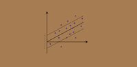
Parameters for to plot the maximum margin separating hyperplane within a two-class separable dataset using a Support Vector Machines classifier with linear kernel

What about leaving the support_ out, which is not defined for a LinearSVC?

import numpy as np
import matplotlib.pyplot as plt
from sklearn import svm

np.random.seed(0)
X = np.r_[np.random.randn(20, 2) - [2, 2], np.random.randn(20, 2) + [2, 2]]
Y = [0] * 20 + [1] * 20

fig, ax = plt.subplots()
clf2 = svm.LinearSVC(C=1).fit(X, Y)

# get the separating hyperplane
w = clf2.coef_[0]
a = -w[0] / w[1]
xx = np.linspace(-5, 5)
yy = a * xx - (clf2.intercept_[0]) / w[1]

# create a mesh to plot in
x_min, x_max = X[:, 0].min() - 1, X[:, 0].max() + 1
y_min, y_max = X[:, 1].min() - 1, X[:, 1].max() + 1
xx2, yy2 = np.meshgrid(np.arange(x_min, x_max, .2),
                     np.arange(y_min, y_max, .2))
Z = clf2.predict(np.c_[xx2.ravel(), yy2.ravel()])

Z = Z.reshape(xx2.shape)
ax.contourf(xx2, yy2, Z, cmap=plt.cm.coolwarm, alpha=0.3)
ax.scatter(X[:, 0], X[:, 1], c=Y, cmap=plt.cm.coolwarm, s=25)
ax.plot(xx,yy)

ax.axis([x_min, x_max,y_min, y_max])
plt.show()

The prediction function $f(\mathbf{z})$ for an SVM model is exactly the signed distance of $\mathbf{z}$ to the separating hyperplane. The separating hyperplane itself is the geometric place $f(\mathbf{z}) = 0$.

For a linear SVM, the separating hyperplane's normal vector $\mathbf{w}$ can be written in input space, and we get:

$$f(\mathbf{z}) = \langle \mathbf{w}, \mathbf{z} \rangle + \rho = \mathbf{w}^T\mathbf{z} + \rho,$$

with $\rho$ the model's bias term.

If a kernel function $\kappa(\mathbf{u},\mathbf{v})=\langle \varphi(\mathbf{u}), \varphi(\mathbf{v})\rangle$ is used, $\mathbf{w}$ typically can no longer be expressed in input space, but only in the space spanned by the embedding function $\varphi(\cdot)$. Then we obtain the following:

$$\begin{align} f(\mathbf{z}) &= \langle \mathbf{w}, \varphi(\mathbf{z})\rangle + \rho = \mathbf{w}^T\varphi(\mathbf{z}) + \rho, \\ &= \sum_{i\in SV} y_i\alpha_i \kappa(\mathbf{x}_i,\mathbf{z}) + \rho, \end{align}$$ with $y$ the vector of labels, $\alpha$ the vector of support values, $\mathbf{x}$'s the support vectors.