You can get the support vectors using clf.support_vectors_.
Plotting the support vectors:
import numpy as np
import matplotlib.pyplot as plt
from sklearn import svm

# we create 40 separable points
np.random.seed(0)
X = np.r_[np.random.randn(20, 2) - [2, 2], np.random.randn(20, 2) + [2, 2]]
Y = [0] * 20 + [1] * 20

# fit the model
clf = svm.SVC(kernel='linear', C=1)
clf.fit(X, Y)

# get the separating hyperplane
w = clf.coef_[0]
a = -w[0] / w[1]
xx = np.linspace(-5, 5)
yy = a * xx - (clf.intercept_[0]) / w[1]


margin = 1 / np.sqrt(np.sum(clf.coef_ ** 2))
yy_down = yy - np.sqrt(1 + a ** 2) * margin
yy_up = yy + np.sqrt(1 + a ** 2) * margin

plt.figure(1, figsize=(4, 3))
plt.clf()
plt.plot(xx, yy, 'k-')
plt.plot(xx, yy_down, 'k--')
plt.plot(xx, yy_up, 'k--')

plt.scatter(clf.support_vectors_[:, 0], clf.support_vectors_[:, 1], s=80,
            facecolors='none', zorder=10, edgecolors='k')
plt.scatter(X[:, 0], X[:, 1], c=Y, zorder=10, cmap=plt.cm.Paired,
            edgecolors='k')

plt.axis('tight')
x_min = -4.8
x_max = 4.2
y_min = -6
y_max = 6

XX, YY = np.mgrid[x_min:x_max:200j, y_min:y_max:200j]
Z = clf.predict(np.c_[XX.ravel(), YY.ravel()])

# Put the result into a color plot
Z = Z.reshape(XX.shape)
plt.figure(1, figsize=(4, 3))
plt.pcolormesh(XX, YY, Z, cmap=plt.cm.Paired)

plt.xlim(x_min, x_max)
plt.ylim(y_min, y_max)

plt.xticks(())
plt.yticks(())

plt.show()

Videos
You can get the support vectors using clf.support_vectors_.
Plotting the support vectors:
import numpy as np
import matplotlib.pyplot as plt
from sklearn import svm

# we create 40 separable points
np.random.seed(0)
X = np.r_[np.random.randn(20, 2) - [2, 2], np.random.randn(20, 2) + [2, 2]]
Y = [0] * 20 + [1] * 20

# fit the model
clf = svm.SVC(kernel='linear', C=1)
clf.fit(X, Y)

# get the separating hyperplane
w = clf.coef_[0]
a = -w[0] / w[1]
xx = np.linspace(-5, 5)
yy = a * xx - (clf.intercept_[0]) / w[1]


margin = 1 / np.sqrt(np.sum(clf.coef_ ** 2))
yy_down = yy - np.sqrt(1 + a ** 2) * margin
yy_up = yy + np.sqrt(1 + a ** 2) * margin

plt.figure(1, figsize=(4, 3))
plt.clf()
plt.plot(xx, yy, 'k-')
plt.plot(xx, yy_down, 'k--')
plt.plot(xx, yy_up, 'k--')

plt.scatter(clf.support_vectors_[:, 0], clf.support_vectors_[:, 1], s=80,
            facecolors='none', zorder=10, edgecolors='k')
plt.scatter(X[:, 0], X[:, 1], c=Y, zorder=10, cmap=plt.cm.Paired,
            edgecolors='k')

plt.axis('tight')
x_min = -4.8
x_max = 4.2
y_min = -6
y_max = 6

XX, YY = np.mgrid[x_min:x_max:200j, y_min:y_max:200j]
Z = clf.predict(np.c_[XX.ravel(), YY.ravel()])

# Put the result into a color plot
Z = Z.reshape(XX.shape)
plt.figure(1, figsize=(4, 3))
plt.pcolormesh(XX, YY, Z, cmap=plt.cm.Paired)

plt.xlim(x_min, x_max)
plt.ylim(y_min, y_max)

plt.xticks(())
plt.yticks(())

plt.show()
Let me assume we are talking about libsvm instead of sklearn svc.
The answer can be found in the LIBLINEAR FAQ. In short, you can't. You need to modify the source code.
Q: How could I know which training instances are support vectors?
Some LIBLINEAR solvers consider the primal problem, so support vectors are not obtained during the training procedure. For dual solvers, we output only the primal weight vector w, so support vectors are not stored in the model. This is different from LIBSVM.
To know support vectors, you can modify the following loop in solve_l2r_l1l2_svc() of linear.cpp to print out indices:
    for(i=0; i<l; i++)
    {
        v += alpha[i]*(alpha[i]*diag[GETI(i)] - 2);
        if(alpha[i] > 0)
            ++nSV;
    }
Note that we group data in the same class together before calling this subroutine. Thus the order of your training instances has been changed. You can sort your data (e.g., positive instances before negative ones) before using liblinear. Then indices will be the same.


Unfortunately there seems to be no way to do that. LinearSVC calls liblinear (see relevant code) but doesn't retrieve the vectors, only the coefficients and the intercept.
One alternative would be to use SVC with the 'linear' kernel (libsvm instead of liblinear based), but also poly, dbf and sigmoid kernel support this option:
from sklearn import svm

X = [[0, 0], [1, 1]]
y = [0, 1]

clf = svm.SVC(kernel='linear')
clf.fit(X, y)
print clf.support_vectors_
Output:
[[ 0.  0.]
 [ 1.  1.]]
liblinear scales better to large number of samples, but otherwise the are mostly equivalent.
I am not sure if it helps, but I was searching for something similar and the conclusion was that when:
clf = svm.LinearSVC()
Then this:
clf.decision_function(x)
Is equal to this:
clf.coef_.dot(x) + clf.intercept_
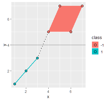
Solving the SVM problem by inspection
By inspection we can see that the boundary decision line is the function $x_2 = x_1 - 3$. Using the formula $w^T x + b = 0$ we can obtain a first guess of the parameters as
$$ w = [1,-1] \ \ b = -3$$
Using these values we would obtain the following width between the support vectors: $\frac{2}{\sqrt{2}} = \sqrt{2}$. Again by inspection we see that the width between the support vectors is in fact of length $4 \sqrt{2}$ meaning that these values are incorrect.
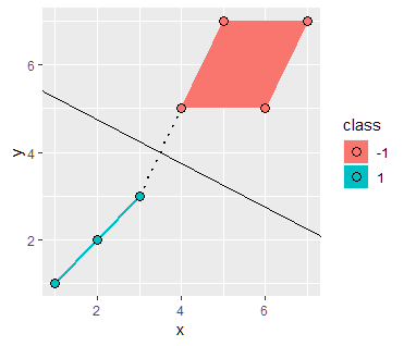
Recall that scaling the boundary by a factor of $c$ does not change the boundary line, hence we can generalize the equation as
$$ cx_1 - xc_2 - 3c = 0$$ $$ w = [c,-c] \ \ b = -3c$$
Plugging back into the equation for the width we get
\begin{aligned} \frac{2}{||w||} & = 4 \sqrt{2} \\ \frac{2}{\sqrt{2}c} & = 4 \sqrt{2} \\ c = \frac{1}{4} \end{aligned}
Hence the parameters are in fact $$ w = [\frac{1}{4},-\frac{1}{4}] \ \ b = -\frac{3}{4}$$
To find the values of $\alpha_i$ we can use the following two constraints which come from the dual problem:
$$ w = \sum_i^m \alpha_i y^{(i)} x^{(i)} $$ $$\sum_i^m \alpha_i y^{(i)} = 0 $$
And using the fact that $\alpha_i \geq 0$ for support vectors only (i.e. 3 vectors in this case) we obtain the system of simultaneous linear equations: \begin{aligned} \begin{bmatrix} 6 \alpha_1 - 2 \alpha_2 - 3 \alpha_3 \\ -1 \alpha_1 - 3 \alpha_2 - 4 \alpha_3 \\ 1 \alpha_1 - 2 \alpha_2 - 1 \alpha_3 \end{bmatrix} & = \begin{bmatrix} 1/4 \\ -1/4 \\ 0 \end{bmatrix} \\ \alpha & = \begin{bmatrix} 1/16 \\ 1/16 \\ 0 \end{bmatrix} \end{aligned}
Source
- https://ai6034.mit.edu/wiki/images/SVM_and_Boosting.pdf
- Full post here
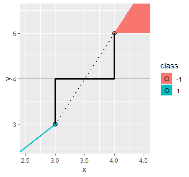
Instead of computing the width between the support vectors (which in this case was easy because two of them happened to be directly across from each other over the decision line), it might be more convenient to use that the support vectors should have value $\pm1$ under the decision function:
$$ cx_1 - cx_2 -3c =0 $$
represents the line, but using the point $B=(2,3)$ with target $-1$ in the diagram, we should have
$$ c(2) - c(3) -3c =-1$$
and hence (again) $c=1/4$.