You can turn the white material transparent:

ImageCompose[img2, ColorReplace[img1, White -> Transparent]]

To change the size, you can ImageResize. Here I have made the resize parameter variable with the slider:

Manipulate[ImageCompose[img2, 
  ImageResize[ColorReplace[img1, White -> Transparent], s]], {s, 50, 300, 1}]

There are also several options for the ImageCompose function and you might try them: you can put the object "on top of" or "xor with", etc.

A good way is to use Inset that you can use to include your image in a Graphics. If you set up the coordinates correctly, you should get correct results.

Everything depends on how you define pixel position meaning if the center of your pixels is on half steps or if you want to have the center on integer positions, but you can adjust this as you like. Let me give a small demo with an 20x20 image:

img = ImageResize[ExampleData[{"TestImage", "Lena"}], {20, 20}];
{nx, ny} = ImageDimensions[img];

Graphics[{
  Inset[img, {1, 1}, {1, 1}, {nx, ny}],
  White, Line[{{2, 2}, {nx - 1, ny - 1}}],
  Green,
  Point[{14.5, 10.5}]
  }, PlotRange -> {{1, nx}, {1, ny}}]

Edit

Long time ago, when Image was in the distant future, the method of displaying pixel data was using Raster. This of course still works and both Inset and Raster will produce a RasterBox in the output expression. Remember that image coordinates have a reversed y-axis and if you use Raster you need to take care of that:

Graphics[{Raster[Reverse@ImageData[img]], White, Green, 
  Table[Point[{i, i}], {i, 1, nx - 1}]}]

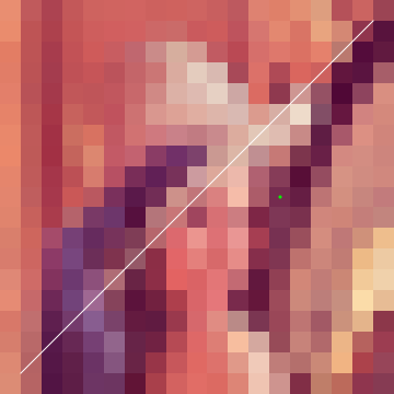
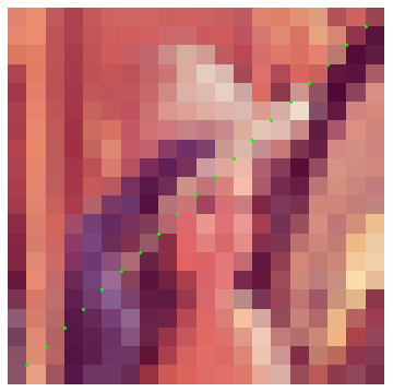
You can use Inset to place the image inside a vector graphics. Inset has various parameters to set the size and position of the image places. To test it you could use a scaled version of an image and overlay it with a grid. You see the lines match exactly:

img = ImageResize[ExampleData[{"TestImage", "Lena"}], {100, 100}];
Graphics[{Inset[img, {0, 0}, {0, 0}, {100, 100}], Line[#], 
    Line[Transpose[#]]}, PlotRange -> {{-1, 101}, {-1, 101}}] &@
 Table[{i, j}, {i, 0, 100, 5}, {j, 0, 100, 5}]

Earth

Using this in your application, you would only have to copy all the code snips:

cart[{lambda_, phi_}] := 
 With[{theta = fc[phi]}, {2/Pi*lambda Cos[theta], Sin[theta]}]
fc[phi_] := 
  Block[{theta}, 
   If[Abs[phi] == Pi/2, phi, 
    theta /. 
     FindRoot[2 theta + Sin[2 theta] == Pi Sin[phi], {theta, phi}]]];

grid = With[{delta = Pi/18/2}, 
   Table[{lambda, phi}, {phi, -Pi/2, Pi/2, delta}, {lambda, -Pi, Pi, 
     delta}]];
gr1 = Graphics[{AbsoluteThickness[0.05], Line /@ grid, 
    Line /@ Transpose[grid]}, AspectRatio -> 1/2];
gr0 = Flatten[{gr1[[1, 2]][[Range[9]*4 - 1]], 
     gr1[[1, 3]][[Range[18]*4 - 3]]}] // 
   Graphics[{AbsoluteThickness[0.2], #}] &;
gr2 = Table[{Hue[t/Pi], Point[{t, t/2}]}, {t, -Pi, Pi, 1/100}] // 
    Flatten // Graphics;
gr = Show[{gr1, gr0, gr2}, Axes -> True];
earthgrid = 
 gr /. Line[pts_] :> {Orange, Line[cart /@ pts]} /. 
  Point[pts_] :> Point[cart[pts]]

Creating an earth-map image

invmollweide[{x_, y_}] := 
 With[{theta = ArcSin[y]}, {Pi x/(2 Cos[theta]), 
   ArcSin[(2 theta + Sin[2 theta])/Pi]}];
img =
 With[{i = 
    Import["https://i.sstatic.net/GaQGa.jpg"]},
  ImageTransformation[i, invmollweide, {512, 256}, 
   DataRange -> {{-Pi, Pi}, {-Pi/2, Pi/2}}, 
   PlotRange -> {{-2, 2}, {-1, 1}}, Padding -> White]
  ];

And then putting all together

Graphics[{Inset[img, {-2, -1}, {0, 0}, {4, 2}], First[earthgrid]}, 
 PlotRange -> {{-2, 2}, {-1, 1}}]

The $over$ operator correctly implemented

According to the Wikipedia, when composing $A$ $over$ $B$, the output alpha channel value $\alpha_O$ and the output color channel value $C_O$ are calculated as follows:

$\begin{cases}\alpha_O = 1 - (1 - \alpha_A) (1 - \alpha_B) \\C_O = \frac{\alpha_A C_A + (1 - \alpha_A)\alpha_B C_B}{\alpha_O}, \text{if $\alpha_O \neq 0$} \\C_O = 0, \text{if $\alpha_O = 0$} \end{cases}$

where $\alpha_A$ and $\alpha_B$ are alpha channel values of $A$ and $B$, and $C_A$ and $C_B$ – color channel values of $A$ and $B$ correspondingly.

This can be directly implemented in Mathematica 11.1 or above as follows:

imageCompose[b_Image, a_Image] := 
 Module[{alphaA = AlphaChannel@a, alphaB = AlphaChannel@b, alphaO, 
         cA = RemoveAlphaChannel@a, cB = RemoveAlphaChannel@b},
  alphaO = 1 - (1 - alphaA) (1 - alphaB);
  SetAlphaChannel[(alphaA*cA + (1 - alphaA) alphaB*cB)/alphaO, alphaO]]

Let us check the associative property:

{{i0, i1, i2}} = ImagePartition[
  Import["https://i.sstatic.net/r13gh.png"], {Scaled[1/3], Scaled[1]}]

{i0~imageCompose~(i1~imageCompose~i2), (i0~imageCompose~i1)~imageCompose~i2}
Equal @@ %
ColorSeparate /@ %%

True

It holds! So what is the problem with ImageCompose of version 10 and later?

Current implementation of ImageCompose: the diagnosis

When writing the above implementation for the first time I unintentionally made a simple mistake: I forgot to divide the output value for the color channel by $\alpha_O$. Here is what happened:

imageComposeWrong[b_Image, a_Image] := 
 Module[{alphaA = AlphaChannel@a, alphaB = AlphaChannel@b, alphaO, 
         cA = RemoveAlphaChannel@a, cB = RemoveAlphaChannel@b},
  alphaO = 1 - (1 - alphaA) (1 - alphaB);
  SetAlphaChannel[alphaA*cA + (1 - alphaA) alphaB*cB, alphaO]]

{i0~imageComposeWrong~(i1~imageComposeWrong~i2), 
 (i0~imageComposeWrong~i1)~imageComposeWrong~i2}
Equal @@ %
ColorSeparate /@ %%

False

The output looks exactly the same as for the current ImageCompose:

{i0~ImageCompose~(i1~ImageCompose~i2), (i0~ImageCompose~i1)~ImageCompose~i2}
Equal @@ %
ColorSeparate /@ %%

False

Numerical comparison reveals tiny differences due to rounding off errors. But the final diagnosis is clear: the developer just forgot to divide the color channel by the alpha channel!

It is a great shame that during more than three years after the release of version 10.0.0 nobody noticed this in the company! Do they themselves use this functionality – or not?!

Please, do not be lazy to report this to the technical support, so that this shameful bug will be fixed as soon as possible! A high priority is given to bugs, which many users write about...

The remedy

From the above considerations the remedy is obvious: we must just divide the color of the ImageCompose output by the alpha channel:

icFix[img_Image] := img/AlphaChannel[img];

{i0~icFix@*ImageCompose~(i1~icFix@*ImageCompose~i2), (i0~icFix@*ImageCompose~i1)~icFix@*ImageCompose~i2}
Subtract @@ % // MinMax
ColorSeparate /@ %%

{-3.10689*10^-6, 3.08454*10^-6}

As one can see, there are still tiny differences due to rounding-off errors, but the associative property in fact is restored and the output is correct!

Original answer

Citing a comment by Rahul:

Well, that's certainly undesirable! Alpha compositing is supposed to be associative (i0~ImageCompose~(i1~ImageCompose~i2) should equal (i0~ImageCompose~i1)~ImageCompose~i2) and this doesn't do that. One could implement correct alpha compositing manually using ImageApply, but let's see if someone has a better way.

Indeed, in versions 8.0.4 and 9.0.1 ImageCompose is associative:

$Version

{{i0, i1, i2}} = ImagePartition[
  Import["https://i.sstatic.net/r13gh.png"], {Scaled[1/3], Scaled[1]}]

{i0~ImageCompose~(i1~ImageCompose~i2), (i0~ImageCompose~i1)~ImageCompose~i2}

Equal @@ %

ColorSeparate /@ %%

"9.0 for Microsoft Windows (64-bit) (January 25, 2013)"

True

... while starting from version 10.0 it is not:

$Version

{{i0, i1, i2}} = ImagePartition[
  Import["https://i.sstatic.net/r13gh.png"], {Scaled[1/3], Scaled[1]}]

{i0~ImageCompose~(i1~ImageCompose~i2), (i0~ImageCompose~i1)~ImageCompose~i2}

Equal @@ %

ColorSeparate /@ %%

"10.0 for Microsoft Windows (64-bit) (September 9, 2014)"

False

It is also worth to note that despite that Overlay[{i0, i1}] and Show[i0, i1] look the same as the old ImageCompose[i0, i1], they are not the same. But they do (approximately) equal to each other and do approximately hold the associative property:

$Version

overlayCompose[i0_, i1_] := Rasterize[Overlay[{i0, i1}], "Image", Background -> None];
showCompose[i0_, i1_] := Rasterize[Show[i0, i1], "Image", Background -> None];

{overlayCompose[i0, i1], showCompose[i0, i1], i0~ImageCompose~i1}

ColorSeparate /@ %

{i0~overlayCompose~(i1~overlayCompose~i2), (i0~overlayCompose~i1)~ overlayCompose~i2}

ColorSeparate /@ %

{i0~showCompose~(i1~showCompose~i2), (i0~showCompose~i1)~showCompose~ i2}

ColorSeparate /@ %

"9.0 for Microsoft Windows (64-bit) (January 25, 2013)"

As one can see from the above, Overlay introduces artifact at the top, while Show does not.

Try this:

(* clip white borders *)
img = ImageCrop[Import["https://i.sstatic.net/La8Zs.jpg"]];

Plot[-14/81 x (x - 18), {x, -2, 19},
     PlotRange -> {-2, 16}, PlotStyle -> Directive[Red, Thick, Dashed], 
     Prolog -> {Texture[img],
                Polygon[{Scaled[{0, 0}], Scaled[{1, 0}], Scaled[{1, 1}], Scaled[{0, 1}]},
                        VertexTextureCoordinates -> {{0, 0}, {1, 0}, {1, 1}, {0, 1}}]},
     Ticks -> None]

Notes:

• If you want to fit in an image as background, you will often want to trim margins; ImageCrop[] is a good function for the purpose.

• Luckily, your background image has its own coordinate system; you can then adjust PlotRange appropriately.

• Prolog is most useful for putting primitives in the background.

• Scaled[] ensures that the background textured polygon is scaled appropriately with respect to the plot range.

The discrepancy arises inside the function Image`CompositionOperationsDump`imvQ in which the ImageSize option value for the graphics is extracted using:

rdims = Cases[i, rul_Rule /; First[rul] === ImageSize];

Since there is no explicit level specification in the Cases it defaults to {1} and therefore when the ImageSize option is at a deeper level (as in your g3) it doesn't get picked up.

It's not clear to me why the code uses Cases here, rather than Options, so I am not sure if this is a bug or a deliberate choice.

 ImageCompose[zePlot, {Graphics[{Blue, Disk[{0, 0}, 5]}, 
  PlotRange -> {{-sqrSize, sqrSize}, {-sqrSize, sqrSize}}], 0.2}]

  ImageCompose[zePlot, {Graphics[{White, Disk[{0, 0}, 5]}, 
  PlotRange -> {{-sqrSize, sqrSize}, {-sqrSize, sqrSize}}, 
  Background -> Blue], 0.2}]

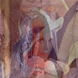
Couldn't you simply Fold ImageCompose onto a list of pairs of layers and blend modes?

Version 7 doesn't have those advanced blend modes as far as I recall, but a simple example using Alpha:

img = ExampleData /@ ExampleData["TestImage"][[25 ;; 27]];

Fold[
 ImageCompose,
 img[[1]],
 {
  {img[[2]], 0.5}, {img[[3]], 0.2}
 }
]