Both formulas are correct. Here is how you can get formula 2, by minimize the sum of squared errors. Dividing it by gives you MSE, and by gives you SSE used in the formula 2. Since you are going to minimize this expression with partial derivation technique, choosing makes the derivation look nice.

Now you use a linear model where and , you get, (I omit the transpose symbol for in ) When you compute its partial derivative over for the additive term, you have,

This is the formula 2 you gave. I don't give the detailed steps, but it is quite straightforward.

Yes, is the activation function, and you do have the factor in the derivative expression as shown above. It disappears if it equals 1, i.e., , where is invariable w.r.t. .

For example, if , (i.e., ), and the prediction model is linear where , too, then you have and .

For another example, if , while the prediction model is sigmoid where , then . This is why in book Artificial Intelligence: A Modern Approach, the derivative of logistic regression is: On the other hand, the formula 1, although looking like a similar form, is deduced via a different approach. It is based on the maximum likelihood (or equivalently minimum negative log-likelihood) by multiplying the output probability function over all the samples and then taking its negative logarithm, as given below,

In a logistic regression problem, when the outputs are 0 and 1, then each additive term becomes,

$$ −logP(y^i|x^i;\theta) = -(y^i\log{h_\theta(x^i)} + (1-y^i)\log(1-h_\theta(x^i))) $$

The formula 1 is the derivative of it (and its sum) when , as below, The derivation details are well given in other post.

You can compare it with equation (1) and (2). Yes, equation (3) does not have the factor as equation (1), since that is not part of its deduction process at all. Equation (2) has additional factors compared to equation (3). Since as probability is within the range of (0, 1), you have , that means equation (2) brings you a gradient of smaller absolute value, hence a slower convergence speed in gradient descent than equation (3).

Note the sum squared errors (SSE) essentially a special case of maximum likelihood when we consider the prediction of is actually the mean of a conditional normal distribution. That is, If you want to get more in depth knowledge in this area, I would suggest the Deep Learning book by Ian Goodfellow, et al.

Maximum Likelihood

Maximum likelihood estimation involves defining a likelihood function for calculating the conditional probability of observing the data sample given probability distribution and distribution parameters. This approach can be used to search a space of possible distributions and parameters.

The logistic model uses the sigmoid function (denoted by sigma) to estimate the probability that a given sample y belongs to class $1$ given inputs $X$ and weights $W$,

\begin{align} \ P(y=1 \mid x) = \sigma(W^TX) \end{align}

where the sigmoid of our activation function for a given $n$ is:

\begin{align} \large y_n = \sigma(a_n) = \frac{1}{1+e^{-a_n}} \end{align}

The accuracy of our model predictions can be captured by the objective function $L$, which we are trying to maximize.

\begin{align} \large L = \displaystyle\prod_{n=1}^N y_n^{t_n}(1-y_n)^{1-t_n} \end{align}

If we take the log of the above function, we obtain the maximum log-likelihood function, whose form will enable easier calculations of partial derivatives. Specifically, taking the log and maximizing it is acceptable because the log-likelihood is monotonically increasing, and therefore it will yield the same answer as our objective function.

\begin{align} \ L = \displaystyle \sum_{n=1}^N t_nlogy_n+(1-t_n)log(1-y_n) \end{align}

In our example, we will actually convert the objective function (which we would try to maximize) into a cost function (which we are trying to minimize) by converting it into the negative log-likelihood function:

\begin{align} \ J = -\displaystyle \sum_{n=1}^N t_nlogy_n+(1-t_n)log(1-y_n) \end{align}

Gradient Descent

Gradient descent is an iterative optimization algorithm, which finds the minimum of a differentiable function. In this process, we try different values and update them to reach the optimal ones, minimizing the output.

Once we have an objective function, we can generally take its derivative with respect to the parameters (weights), set it equal to zero, and solve for the parameters to obtain the ideal solution. However, in the case of logistic regression (and many other complexes or otherwise non-linear systems), this analytical method doesn’t work. Instead, we resort to a method known as gradient descent, whereby we randomly initialize and then incrementally update our weights by calculating the slope of our objective function. When applying the cost function, we want to continue updating our weights until the slope of the gradient gets as close to zero as possible. We can show this mathematically:

\begin{align} \ w:=w+\triangle w \end{align}

where the second term on the right is defined as the learning rate times the derivative of the cost function with respect to the weights (which is our gradient):

\begin{align} \ \triangle w = \eta\triangle J(w) \end{align}

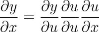
Thus, we want to take the derivative of the cost function with respect to the weight, which, using the chain rule, gives us:

\begin{align} \frac{J}{\partial w_i} = \displaystyle \sum_{n=1}^N \frac{\partial J}{\partial y_n}\frac{\partial y_n}{\partial a_n}\frac{\partial a_n}{\partial w_i} \end{align}

Thus, we are looking to obtain three different derivatives. Let us start by solving for the derivative of the cost function with respect to $y$:

\begin{align} \frac{\partial J}{\partial y_n} = t_n \frac{1}{y_n} + (1-t_n) \frac{1}{1-y_n}(-1) = \frac{t_n}{y_n} - \frac{1-t_n}{1-y_n} \end{align}

Next, let us solve for the derivative of $y$ with respect to our activation function:

\begin{align} \large y_n = \sigma(a_n) = \frac{1}{1+e^{-a_n}} \end{align}

\begin{align} \frac{\partial y_n}{\partial a_n} = \frac{-1}{(1+e^{-a_n})^2}(e^{-a_n})(-1) = \frac{e^{-a_n}}{(1+e^-a_n)^2} = \frac{1}{1+e^{-a_n}} \frac{e^{-a_n}}{1+e^{-a_n}} \end{align}

\begin{align} \frac{\partial y_n}{\partial a_n} = y_n(1-y_n) \end{align}

And lastly, we solve for the derivative of the activation function with respect to the weights:

\begin{align} \ a_n = W^TX_n \end{align}

\begin{align} \ a_n = w_0x_{n0} + w_1x_{n1} + w_2x_{n2} + \cdots + w_Nx_{NN} \end{align}

\begin{align} \frac{\partial a_n}{\partial w_i} = x_{ni} \end{align}

Now we can put it all together and simply.

\begin{align} \frac{\partial J}{\partial w_i} = - \displaystyle\sum_{n=1}^N\frac{t_n}{y_n}y_n(1-y_n)x_{ni}-\frac{1-t_n}{1-y_n}y_n(1-y_n)x_{ni} \end{align}

\begin{align} = - \displaystyle\sum_{n=1}^Nt_n(1-y_n)x_{ni}-(1-t_n)y_nx_{ni} \end{align}

\begin{align} = - \displaystyle\sum_{n=1}^N[t_n-t_ny_n-y_n+t_ny_n]x_{ni} \end{align}

\begin{align} \frac{\partial J}{\partial w_i} = \displaystyle\sum_{n=1}^N(y_n-t_n)x_{ni} = \frac{\partial J}{\partial w} = \displaystyle\sum_{n=1}^{N}(y_n-t_n)x_n \end{align}

We can get rid of the summation above by applying the principle that a dot product between two vectors is a summover sum index. That is:

\begin{align} \ a^Tb = \displaystyle\sum_{n=1}^Na_nb_n \end{align}

Therefore, the gradient with respect to w is:

\begin{align} \frac{\partial J}{\partial w} = X^T(Y-T) \end{align}

If you are asking yourself where the bias term of our equation (w0) went, we calculate it the same way, except our x becomes 1.

• Deep Learning Prerequisites: Logistic Regression in Python
• Logistic Regression using Gradient descent and MLE (Projection)
• Logistic Regression.pdf
• Maximum likelihood and gradient descent
• MAXIMUM LIKELIHOOD ESTIMATION (MLE)
• Stanford.edu-Logistic Regression.pdf
• Gradient Descent Equation in Logistic Regression