


First, there is no need to use Module in your sample code above. You could write simply:
CCGray[pic_?ImageQ] := ColorConvert[pic,"GrayScale"]
Now, if you want to manage the channel mixing manually you can use ImageApply and Dot:
customGray[img_?ImageQ, ker_?VectorQ] := ImageApply[ker.# &, img]

img = Import["https://i.sstatic.net/wtlqF.jpg"];

customGray[img, {0.8, 0.5, -0.3}]

You'll notice that my three values add to one; this is typically necessary to preserve white as white. If you want to make this automatic just divide by the total:
customGray2[img_?ImageQ, ker_?VectorQ] := With[{k = ker/Tr@ker}, ImageApply[k.# &, img]]
Or with normalization control as an Option:
Options[customGray2] = {Normalize -> True};

customGray2[img_?ImageQ, ker_?VectorQ, OptionsPattern[]] :=
  With[{k = If[OptionValue[Normalize], ker/Tr@ker, ker]},
    ImageApply[k.# &, img]
  ]
This makes it easy to Manipulate:
Manipulate[
 customGray2[img, {a, b, c}],
 {a, -5, 5}, {b, -5, 5}, {c, -5, 5}
]

First, there is no need to use Module in your sample code above. You could write simply:
CCGray[pic_?ImageQ] := ColorConvert[pic,"GrayScale"]
Now, if you want to manage the channel mixing manually you can use ImageApply and Dot:
customGray[img_?ImageQ, ker_?VectorQ] := ImageApply[ker.# &, img]

img = Import["https://i.sstatic.net/wtlqF.jpg"];

customGray[img, {0.8, 0.5, -0.3}]
You'll notice that my three values add to one; this is typically necessary to preserve white as white. If you want to make this automatic just divide by the total:
customGray2[img_?ImageQ, ker_?VectorQ] := With[{k = ker/Tr@ker}, ImageApply[k.# &, img]]
Or with normalization control as an Option:
Options[customGray2] = {Normalize -> True};

customGray2[img_?ImageQ, ker_?VectorQ, OptionsPattern[]] :=
  With[{k = If[OptionValue[Normalize], ker/Tr@ker, ker]},
    ImageApply[k.# &, img]
  ]
This makes it easy to Manipulate:
Manipulate[
 customGray2[img, {a, b, c}],
 {a, -5, 5}, {b, -5, 5}, {c, -5, 5}
]
I assume you've rejected this option:
BubbleChart[RandomReal[{-1, 1}, {10, 5, 3}],
  ColorFunction -> "GrayTones"]

I believe the best way to make this conversion is to use ImageApply and Dot:
img = Import["ExampleData/lena.tif"]

ImageApply[{.3, .5, .2}.# &, img]

Please ask your future questions on the dedicated Mathematica StackExchange site:

This works and is more Mathematica style code.
SetDirectory[NotebookDirectory[]];
img = Import["55th-All-Japan-Kendo-Champ2007-4.jpg"];
colorXform[p_] := p[[1]]*0.3 + p[[2]]*0.5 + p[[3]]*0.2;
newImg = Image[Map[colorXform, ImageData[img], {2}]];
Show[newImg]
We can obtain the exact values used by mathematica by making up a 3 pixel image with pure red,green,blue and converting it:
 lvec = First@
         ImageData[
           ColorConvert[Image[{{{1, 0, 0}, {0, 1, 0}, {0, 0, 1}}}],
             "GrayScale"]]
{0.299, 0.587, 0.114}
Note these are the "Rec. 601 luna coefficients" per http://en.wikipedia.org/wiki/Luma_%28video%29
Test this on a real image:
 lena = ExampleData[{"TestImage", "Lena"}];
 lenag = ColorConvert[lena, "GrayScale"];
 ImageData@ImageApply[ lvec.# & , lena ] == ImageData@lenag
True
See How can I convert colors to grayscale? for insight into how the calculation might be being done.
The two images produced by the commands below are a close match, but you could figure out the exact scaling vector with a short program making multiple comparisons. A further test on a different image would ascertain whether ColorConvert uses the same vector all the time, or whether the image is analysed before conversion for an optimal grayscale appearance.
ColorConvert[img, "GrayScale"]

ImageApply[{0.35, 0.45, 0.2}.# &, img]
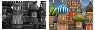
Using the images in the duplicate question,
grey = Import["hstbasils.jpg"];
colour = Import["St.-Basils-Cathedral-001.jpg"];
{grey, colour}
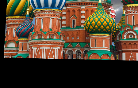
transform = Last@FindGeometricTransform[colour, grey];
tcolour =
 ImageTransformation[colour, transform, DataRange -> Full,
  PlotRange -> Transpose@{{0, 0}, ImageDimensions@grey}];
ColorCombine[{First@ColorSeparate[grey, "LAB"]}~Join~
  Rest@ColorSeparate[tcolour, "LAB"], "LAB"]
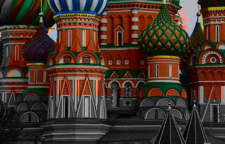
It's not perfect, but it's something.
Here is one approach that does not respect object boundaries that uses HistogramTransform` in the HSB color space. For example, you can colorize the black and white image imgBW (according to the colors in the reference image img) using:
img = Import["http://static.guim.co.uk/sys-images/Guardian/Pix/pictures/2012/3/14/1331719456752/St.-Basils-Cathedral-001.jpg"];
imgBW = Import["http://fc06.deviantart.net/fs71/f/2012/047/6/b/saint_basil__s_cathedral_by_tomdal-d4pwlwo.jpg"];

HistogramTransform[ColorConvert[imgBW, "HSB"], ColorConvert[img, "HSB"]]
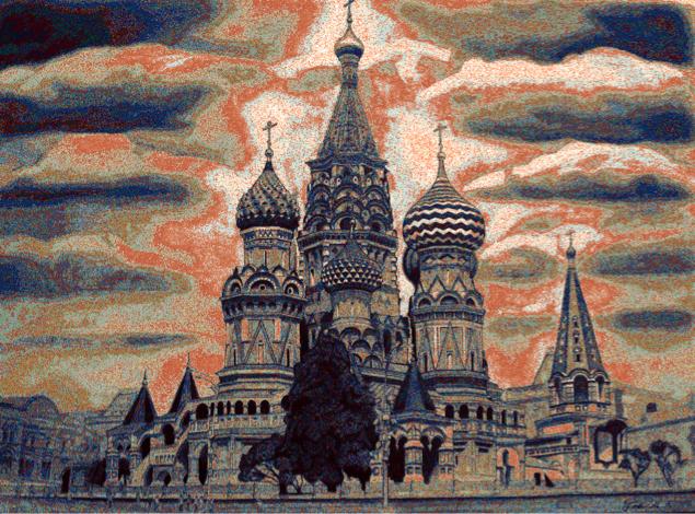
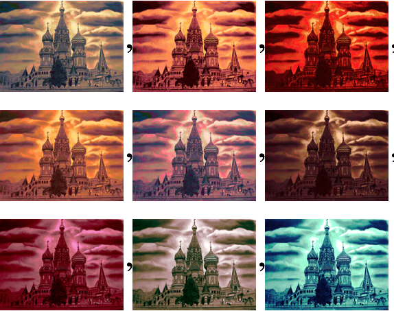
which is a colorful if inauthentic colorization. You can also try the same thing in "LAB" and the other colorspaces.
There is no need to apply the histogram transformations to the same channel in the various images. Here is the application of all the different color spaces, and a sampling of the output.
fun[{x_, y_}] := HistogramTransform[ColorConvert[imgBW, x], ColorConvert[img, y]];
colSpaces = {"LAB", "RGB", "HSB", "LCH", "LUV", "XYZ"};
allCols = Flatten[Outer[List, colSpaces, colSpaces], 1];
fun[#] & /@ allCols
One way would be to use ColorConvert to convert the RGB or Hue values to gray scale. Here's an example:
Plot[{Sin[x], Cos[x], Exp[-x^2], Sinc[π x]}, {x, 0, π}] /.
  x : _RGBColor | _Hue | _CMYKColor :> ColorConvert[x, "Grayscale"]


For 2D plots that accept a ColorFunction, you can simply use GrayLevel to get the plot in grayscale as:
DensityPlot[
  Sin[x ^2 + y^2], {x, 0, 3}, {y, 0, 3},
  ColorFunction -> GrayLevel,
  PlotPoints -> 100
]


Typically, these grayscale plots are useful when submitting to journals that charge exorbitant prices just to print in colour. However, just a note of caution that discerning different shades of gray is not easy. For the most effect, it is recommended (at least in the journals I publish in), that you also change the line type for your different curves (and not more than 4 curves/plot). You should also choose the colours (or colourscale, for 2D surface plots) wisely so that they convert well to grayscale. For example:


One way would be to roll your own color functions. For continuous use:
grayScale = Blend[{Black, White}, #1] &

ContourPlot[Sin[x + y], {x, 0, 2 \[Pi]}, {y, 0, \[Pi]},
  ColorFunction -> grayScale]

For discrete plots:
grayColorList = (Blend[{Black, White}, #] & /@ Range[0, 1, 0.1])

Plot[Sin[x], {x, 0, 2 \[Pi]}, PlotStyle -> grayColorList[[1]]]

Using ND is not necessary, as Mathematica makes it easy to construct InterpolatingFunction objects, which can then be formally differentiated using Derivative. First, a sample image:
data = Import[
  "http://41.media.tumblr.com/bece7ed81870c8e9b904290700451eb2/tumblr_\
mv8m2sE2FW1slvzano1_400.jpg"]

Convert to grayscale, and then convert the resulting matrix into an InterpolatingFunction object:
imData = ImageData[ColorConvert[data, "Grayscale"]];
f = ListInterpolation[imData];
Plot the InterpolatingFunction using DensityPlot:
DensityPlot[f[-x, y], {y, 1, 400}, {x, -1, -398}, PlotPoints -> 300,
 ColorFunction -> GrayLevel]

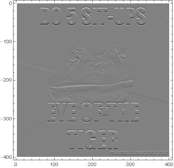
Plot the first partial derivative in the $x$-direction:
g = Derivative[1, 0][f];
DensityPlot[g[-x, y], {y, 1, 400}, {x, -1, -398}, PlotPoints -> 300,
 PlotRange -> All, ColorFunction -> GrayLevel]
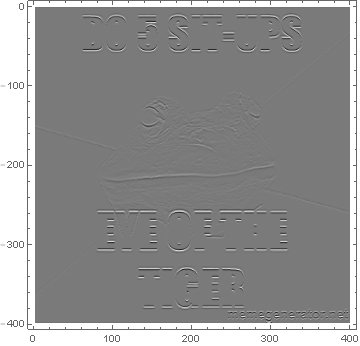
Plot the second partial derivative in the $x$-direction:
h = Derivative[2, 0][f];
DensityPlot[h[-x, y], {y, 1, 400}, {x, -1, -398}, PlotPoints -> 300,
 PlotRange -> All, ColorFunction -> GrayLevel]
Of course, you can get better results with even less work by using bill s's answer.
You can get the values of the pixel intensities directly using the built-in functions PixelValue and/or ImageValue. For example, using DumpsterDoofus's image, the RGB pixel values at location {100,100} are easy to find, and their mean is (roughly) the intensity.
data = Import["http://41.media.tumblr.com/bece7ed81870c8e9b904290700451eb2/tumblr_mv8m2sE2FW1slvzano1_400.jpg"];
PixelValue[data, {100, 100}]
Mean[PixelValue[data, {100, 100}]]
Depending on what you want to do with the image, there may be no need to do the interpolation at all. There are many functions that deal directly with images, including GradientFilter (that does more or less what you ask for in a single command). If your goal in taking the derivatives is to detect edges, then there is Edgedetect. GradientOreintationFilter is another option.
GradientFilter[data, {2, 0.1}]

You can take the second derivative
GradientFilter[GradientFilter[data, {1, 0.1}], {1, 0.1}]
and there are numerous options to control the process.
im1 = Import["http://www.furnituremaker.com/images/Craftsman.gif"]
Perhaps something like this?
ColorNegate@Binarize@ImageResize[im1, Scaled[4]]~Image~
 ImageType[im1]~ImageResize~ImageDimensions[im1]

(thanks to @RahulNarain's for his suggestions)
A fun new command in Mathematica 9 is ColorReplace:
ColorReplace[im1, {Black -> White, Brown -> Black}]

You could probably play with these and Blur functions too to get the results you want. (I guessed at Brown... :)
Here's one way:
data = RandomReal[{0, 1}, {100, 100}];
ColorCombine[{Image[data], Image[0 data], Image[0 data]}]

This creates an RGB image which has the data as the Red channel, and all zeros in the Green and Blue channels. By weighting them differently you can get any color you wish. For instance, you can get yellow:
ColorCombine[{Image[data], Image[data], Image[0 data]}]

For this purpose you can use the function Colorize which is sufficient even for fancy coloring. Let's make some examples with a B&W photo
img = Import["https://i.sstatic.net/397vv.png"]

If you simply want to use the gray channel as one or more color channels you use
Colorize[img, ColorFunction -> Function[gray, RGBColor[0, gray, gray]]]

The same works of course with other color functions
Colorize[img, ColorFunction -> Function[gray, Hue[0.6, 1 - gray, gray]]]

With the built-in color schemes of Mathematica you can get more fancy looks and the usage is even simpler
Colorize[img, ColorFunction -> "AvocadoColors"]

Or you mix everything together
Colorize[img, ColorFunction ->
  Function[gray, RGBColor @@ (gray*List @@ ColorData["BrightBands", gray])]]

im = ExampleData[{"TestImage", "Aerial"}];

Colorize[im, ColorFunction -> "AvocadoColors"] // Timing // First
(* 0.093750 *)
versus
ImageApply[List @@ ColorData["AvocadoColors"][#] &, im] // Timing // First
(* 0.265625 *)

ImageApply[List @@ Blend["AvocadoColors", #] &, im] // Timing // First (thanks: @Kuba *)
(* 0.109375 *)
For a larger image:
imlarge = Image[ RandomReal[1, {1080, 1920}]];

f1 = Colorize[#, ColorFunction -> "AvocadoColors"] &;
f2 = Image@Raster[ImageData[#, DataReversed -> True], ColorFunction -> "AvocadoColors"] &;
f3 = ImageApply[List @@ Blend["AvocadoColors", #] &, #] &;

First[Timing@#[imlarge]] & /@ {f1, f2, f3}
{2.234375, 2.140625, 3.093750}
Raster will be helpful, as it has the ColorFunction option and it can be directly converted back to an Image.
Let img be a grayscale image:
img = ColorConvert[ExampleData[{"TestImage", "Lena"}], "Grayscale"]

Image@Raster[ImageData[img, DataReversed -> True], ColorFunction -> "Rainbow"]
