![{\displaystyle \Pr[Y=m]=\sum _{k=m}^{n}{\binom {n}{m}}{\binom {n-m}{k-m}}p^{k}q^{m}(1-p)^{n-k}(1-q)^{k-m}}](https://imgs.search.brave.com/_ZzMOmRKyfxVmQ4vVVgLsklO2iEaHy6xvZBCUdfHG-4/rs:fit:500:0:0:0/g:ce/aHR0cHM6Ly93aWtp/bWVkaWEub3JnL2Fw/aS9yZXN0X3YxL21l/ZGlhL21hdGgvcmVu/ZGVyL3N2Zy84MzY5/ZWY4NDZmZmRhNzI5/MDBlZmM2N2IzMzQ5/MjNmNzBjZTQ4Y2E1.jpeg)
Factsheet
Videos
What is the mean value of binomial distribution?
What are the parameters of a Binomial Distribution?
What are the applications of Binomial Distribution?
Let  , where
  is a constant. Then
 Differentiate with respect to
  . We get
 Multiply through by
  , and set
  .
.
Remark: Here is a nicer proof. Let random variable  be equal to
  if there is a success on the
  -th trial, and let
  otherwise. Then our binomial random variable
  is equal to
  . By the linearity of expectation we have
  . Each
  has expectation
  , so
, so  .
.
Ugh, that's a nasty way to do it! The steps are correct, but the starting point is wrong; it just happens to work in this case.
Consider instead
 This is called the Probability Generating Function of the random variable
  . It has some properties that are easy to relate to properties of
  : the most basic of these is probably
 Now, what happens when we differentiate?
 so
so
 Ah, this is what we want. You can go further and derive an expression for the variance, but that's not what we're interested in here. For the binomial distribution, it is easy to see using the binomial theorem that
 Ah, no this looks rather like the starting point of your expression, but we have a
  in it as well. Hence we have a free variable with respect to which we can differentiate:

Any discrete probability distribution has a generating function, and exactly the same technique can be applied: that's why this idea's useful.
It's good to be able to do the calculations. It's also good to know other ways to get the answer, so here is one.
A variable with binomial distribution with parameters  and
and  is equivalent to the sum of
  independent Bernoulli variables with parameter
  (variables that have value
  with probability
  ,
,  otherwise). This models the number of heads in
  tosses of a (possibly unfair) coin. You might even say this is the motivation for the definition of the binomial distribution.
To see why the sum of  i.i.d. Bernoulli variables and the binomial distribution are equivalent, let
  be the number of heads in
  tosses of a coin that comes up heads with probability
  and consider the probability that you have exactly
  heads.
(That is,
heads.
(That is,  "success" outcomes in
  Bernoulli variables with parameter
  .)
Any particular sequence of
.)
Any particular sequence of  heads and
  tails has probability
 , and there are
  sequences of
  heads and
  tails. Therefore
 so
so  has a binomial distribution by definition.
So we can define  i.i.d. Bernoulli variables
  such that
  , and then
  has a binomial distribution with parameters
  and
and  .
.
The expected value (mean) of the Bernoulli variable  is
is  .
By the linearity of expectation, the expected value of the sum of the
.
By the linearity of expectation, the expected value of the sum of the  Bernoulli variables (that is, the expected value of
  )
is the sum of their expected values,
)
is the sum of their expected values,

As a bonus of this method of proof, we also have a formula for the distribution of a sum of Bernoulli variables, which is often the source of a binomial distribution.
I think I was able to solve my own problem.
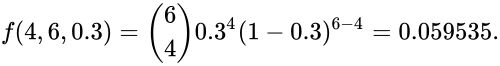
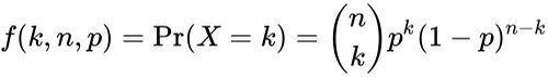
The Binomial Distribution is defined as:

And from first principles, the Expected Value of the Binomial Distribution can be written as:

Note that this sum can be written from  , since
  makes no contribution to this sum:

Now, let's open the Binomial Coefficient :

Now for some simplifications - remember that we can write  as
as  . This means that we can write
  and
and  . Using this information, we can re-write the above term as:

We can see that the first  and the
  in the denominator cancel out. Also note that
  can be written as
  . So now, we can write:

We can see an  in the above term that is not contributing to the sum - therefore, we can take it outside:

Now, let define a new variable  . This means that we can re-write the above expression as:

Next, we can see that  is in the form of a Binomial Coefficient
  . So now, we can write:

And finally, we can notice that the summation term is of the form:  . Using this logic, we can write the above term as:


Thus, we have shown that

Am I correct?
I find this term annoying because in my head n*p refers to the expected value and not the mean of a sample.
Say if we had a coin flip where x=number of heads, we know that the expected value of each coin flip is 0.5 heads and so the expected value of a 100 coin flip is 50 heads aka 100 * 0.5.
When we carry out an experiment we know that as N gets larger we expect that the average amount of heads per coin flip will approach 0.5 ie (n*p)/n, this is the mean that it's approaching. So why then do people refer to n*p is the mean of the data in binomial distributions? n*p doesn't approach anything as n gets bigger as the result just gets bigger as well?