You can interpolate your data using scipy's 1-D Splines functions. The computed spline has a convenient derivative method for computing derivatives.
For the data of your example, using UnivariateSpline gives the following fit
import matplotlib.pyplot as plt
from scipy.interpolate import UnivariateSpline

y_spl = UnivariateSpline(x,y,s=0,k=4)

plt.semilogy(x,y,'ro',label = 'data')
x_range = np.linspace(x[0],x[-1],1000)
plt.semilogy(x_range,y_spl(x_range))

The fit seems reasonably good, at least visually. You might want to experiment with the parameters used by UnivariateSpline.
The second derivate of the spline fit can be simply obtained as
y_spl_2d = y_spl.derivative(n=2)

plt.plot(x_range,y_spl_2d(x_range))

The outcome appears somewhat unnatural (in case your data corresponds to some physical process). You may either want to change the spline fit parameters, improve your data (e.g., provide more samples, perform less noisy measurements), or decide on an analytic function to model your data and perform a curve fit (e.g., using sicpy's curve_fit)
You can interpolate your data using scipy's 1-D Splines functions. The computed spline has a convenient derivative method for computing derivatives.
For the data of your example, using UnivariateSpline gives the following fit
import matplotlib.pyplot as plt
from scipy.interpolate import UnivariateSpline

y_spl = UnivariateSpline(x,y,s=0,k=4)

plt.semilogy(x,y,'ro',label = 'data')
x_range = np.linspace(x[0],x[-1],1000)
plt.semilogy(x_range,y_spl(x_range))
The fit seems reasonably good, at least visually. You might want to experiment with the parameters used by UnivariateSpline.
The second derivate of the spline fit can be simply obtained as
y_spl_2d = y_spl.derivative(n=2)

plt.plot(x_range,y_spl_2d(x_range))
The outcome appears somewhat unnatural (in case your data corresponds to some physical process). You may either want to change the spline fit parameters, improve your data (e.g., provide more samples, perform less noisy measurements), or decide on an analytic function to model your data and perform a curve fit (e.g., using sicpy's curve_fit)
By finite differences, the first order derivative of y for each mean value of x over your array is given by :
dy=np.diff(y,1)
dx=np.diff(x,1)
yfirst=dy/dx
And the corresponding values of x are :
xfirst=0.5*(x[:-1]+x[1:])
For the second order, do the same process again :
dyfirst=np.diff(yfirst,1)
dxfirst=np.diff(xfirst,1)
ysecond=dyfirst/dxfirst

xsecond=0.5*(xfirst[:-1]+xfirst[1:])
How To Take Derivatives In Python: 3 Different Types of Scenarios
Higher order central differences using NumPy.gradient()
python - Computing numeric derivative via FFT - SciPy - Computational Science Stack Exchange
scipy - Implementation of the second derivative of a normal probability distribution function in python - Stack Overflow
Videos
Ndimage generates a Gaussian kernel by sampling a Gaussian and normalizing it to 1. The derivative of this kernel is generated by modifying that normalized kernel according to the chain rule to compute the derivative, and this modification is applied repeatedly to obtain higher order derivatives. Here is the relevant source code.
This indeed leads to a kernel that produces imprecise second order derivatives, as described by the OP in the question and the very nice answer.
Indeed, one can not just sample a derivative of Gaussian to obtain a convolution kernel, because the Gaussian function is not band-limited, and so sampling causes aliasing. The Gaussian function is nearly bandlimited, sampling with a sample spacing of  leads to less than 1% of the energy being aliased. But as the order of the derivative increases, so does the bandlimit, meaning that the higher the derivative order, the more sampling error we get. [Note that if we had no sampling error, convolution with the sampled kernel would yield the same result as a convolution in the continuous domain.]
So we need some tricks to make the Gaussian derivatives more precise. In DIPlib (disclosure: I'm an author) the second order derivative is computed as follows (see the relevant bit of source code):
- Sample the second order derivative of the Gaussian function.
- Subtract the mean, to ensure that the response to a contant function is 0.
- Normalize such that the kernel, multiplied by a unit parabola (
 ), sums to 2, to ensure that the response to a parabolic function has the right magnitude.
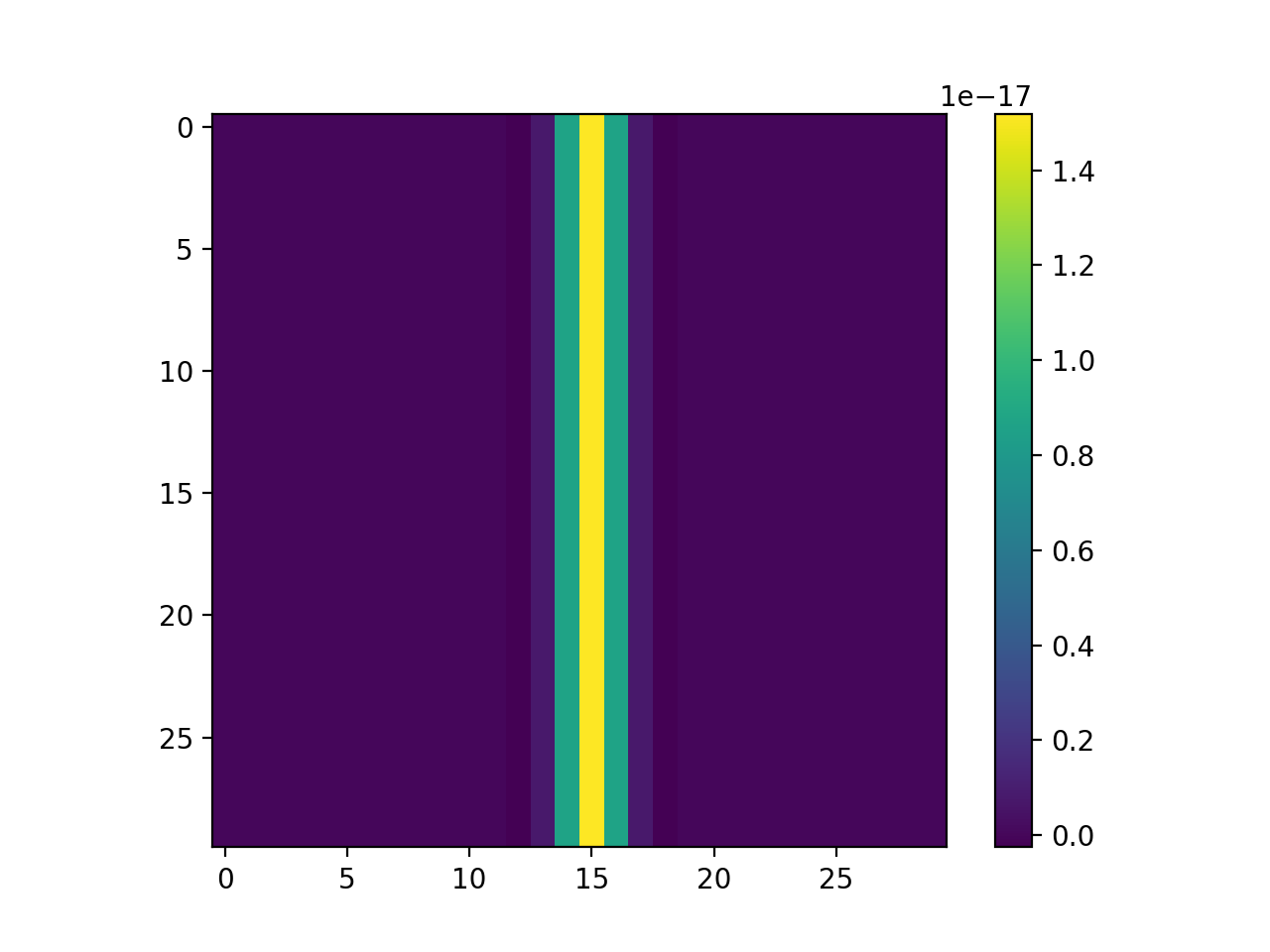
As we can see, the error in this case is within numerical precision of the double-precision floating-point values:
import diplib as dip
import numpy as np
import matplotlib.pyplot as plt

A = np.zeros((30,30))
A[:,15] = 1

B = dip.Gauss(A, [1], [0,2])  # note dimension order is always [x,y] in DIPlib

plt.imshow(B)
plt.colorbar()
plt.show()
The DIPlib code to generate a 1D second order derivative of the Gaussian is equivalent to the following Python code:
import numpy as np

sigma = 2.0
radius = np.ceil(4.0 * sigma)

x = np.arange(-radius, radius+1)
g = np.exp(-(x**2) / (2.0 * sigma**2)) / (np.sqrt(2.0 * np.pi) * sigma)
g2 = g * (x**2 / sigma**2 - 1) / sigma**2
g2 -= np.mean(g2)
g2 /= np.sum(g2 * x**2) / 2.0
I think I have figured out the answer. The results have to do with the difference between the integral of a continuous Gaussian function, versus the sum of a discretized Gaussian.
In the ideal case, continuous and discrete sums of Gaussians already differ
As one illustrative example, consider the integral of a Gaussian versus the discrete summation of a Gaussian with unit steps is
$$ \int_{-\infty}^\infty e^{-x^2}\!\text{d}x=\sqrt{\pi}\approx 1.77245,\qquad \sum_{x\in\mathbb{Z}} e^{-x^2} = \theta_3(0,e^{-1})\approx 1.77264.$$
Apparently, the two expressions differ in the details (after 4 decimals). Such things matter when we compare a continuous convolution ( ) against a discrete convolution (
 ) using Gaussian kernels.
Symmetric versus asymmetric functions
A Gaussian is a symmetric function, i.e.,  . The first derivative of a Gaussian is antisymmetric, i.e.,
  . The second derivative of a Gaussian is symmetric again, and so on.
Implication for convolutions
We consider truncated (to  terms, although we include
  in this description) convolutions with Gaussians
  or their
  -th derivatives (
 ) with the following computation:
 Knowing that Gaussian functions are either anti-symmetric or symmetric, that means we can 'simplify' the summation to only consider non-negative integer values for
  ,
,

We now note that for an odd (i.e., first-order, third-order, ...) derivative of a Gaussian, the antisymmetry also implies that  . This is not true for an even derivative of a Gaussian, where
  .
.
Specific example for constant functions, 
We can thus symbolically write down what happens when convolving a Gaussian derivative with a constant function  . For a first derivative, with
  , we compute
 that is, it evaluates to 0, which we expect from differentiating a constant function.
Conversely, for a second derivative,  , it results in
 This expression only equals the expected result of 0, if the truncated and discrete kernel
  sums to 0, which is alternatively expressed as the expression above. This strict requirement is not met for discrete sums of a Gaussian derivative, even without truncation (i.e., when letting
  the sum is still not 0)!
Explaining the observed behavior
So, I can now answer the question posed above (which was 'why do two successive 1st-order derivatives give the correct result, but a single 2nd-order derivative not?'): after applying the first derivative operation, only zeroes remain (per the result for  described above), which leads to field of zeroes for the second convolution operation. Conversely, an immediate application of
  simply returns the sum of the kernel
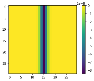
  multiplied with the local value. That second definition should be 0 in the ideal and continuous case -- but because we're working with a discrete application of convolutions it ceases to hold. Even if we use a very large truncation (e.g., specify
 truncate=1000 when calling the Gaussian filter in Python), it will not converge to 0. Instead, it will converge to  (the term
  comes from the Gaussian which is applied in the horizontal direction), which we can confirm with our code:
import numpy as np
import matplotlib.pyplot as plt
A = np.zeros((30,30))
A[:,15] = 1
from scipy.ndimage import gaussian_filter
B = gaussian_filter(A, sigma=1, order=[2, 0], mode='reflect', truncate=10000)
plt.imshow(B)
plt.colorbar()
plt.show()
print(B[0,15]) # >> -8.426948379372423e-08
So, to conclude, the scipy implementation is correct, and it does what it is supposed to do, from a discrete point of view. However, from a continuous point of view, the results are slightly unexpected and seem wrong. I'll ponder what the most appropriate fix is. Perhaps, we must simply ensure that the summation convention holds, by slightly modifying the kernel  , after which the discrete kernel will mimic the continuous kernel, at least for constant functions!
FFT returns a complex array that has the same dimensions as the input array. The output array is ordered as follows:
Element 0 contains the zero frequency component, F0.
The array element F1 contains the smallest, nonzero positive frequency, which is equal to 1/(Ni Ti), where Ni is the number of elements and Ti is the sampling interval.
F2 corresponds to a frequency of 2/(Ni Ti).
Negative frequencies are stored in the reverse order of positive frequencies, ranging from the highest to lowest negative frequencies.
For an even number of points, the frequencies corresponding to the returned complex values are: 0, 1/(NiTi), 2/(NiTi), ..., (Ni/2–1)/(NiTi), 1/(2Ti), –(Ni/2–1)/(NiTi), ..., –1/(NiTi) where 1/(2Ti) is the Nyquist critical frequency.
For an odd number of points, the frequencies corresponding to the returned complex values are: 0, 1/(NiTi), 2/(NiTi), ..., (Ni–1)/2)/(NiTi), –(Ni–1)/2)/(NiTi), ..., –1/(NiTi)
Using this information we can construct the proper vector of frequencies that should be used for calculating the derivative. Below is a piece of self-explanatory Python code that does it all correctly. Note that the factor 2$\pi$N cancels out due to normalization of FFT.
from scipy.fftpack import fft, ifft, dct, idct, dst, idst, fftshift, fftfreq
from numpy import linspace, zeros, array, pi, sin, cos, exp, arange
import matplotlib.pyplot as plt


N = 100
x = 2*pi*arange(0,N,1)/N #-open-periodic domain

dx = x[1]-x[0]
y = sin(2*x)+cos(5*x)
dydx = 2*cos(2*x)-5*sin(5*x)


k2=zeros(N)

if ((N%2)==0):
    #-even number
    for i in range(1,N//2):
        k2[i]=i
        k2[N-i]=-i
else:
    #-odd number
    for i in range(1,(N-1)//2):
        k2[i]=i
        k2[N-i]=-i

dydx1 = ifft(1j*k2*fft(y))

plt.plot(x,dydx,'b',label='Exact value')
plt.plot(x,dydx1, color='r', linestyle='--', label='Derivative by FFT')
plt.legend()
plt.show()

Maxim Umansky’s answer describes the storage convention of the FFT frequency components in detail, but doesn’t necessarily explain why the original code didn’t work. There are three main problems in the code:
x = linspace(0,2*pi,N): By constructing your spatial domain like this, yourxvalues will range from $0$ to $2\pi$, inclusive! This is a problem because your functiony = sin(2*x)+cos(5*x)is not exactly periodic on this domain ($0$ and $2\pi$ correspond to the same point, but they’re included twice). This causes spectral leakage and thus a small deviation in the result. You can avoid this by usingx = linspace(0,2*pi,N, endpoint=False)(orx = 2*pi*arange(0,N,1)/N, as Maxim Umansky did; this is what he is referring to with “open-periodic domain”).k = fftshift(k): As Maxim Umansky explained, yourkvalues need to be in a specific order to match the FFT convention.fftshiftsorts the values (from small/negative to large/positive), which can be useful e. g. for plotting, but is incorrect for computations.dydx1 = ifft(-k*1j*fft(y)).real:scipydefines the FFT asy(j) = (x * exp(-2*pi*sqrt(-1)*j*np.arange(n)/n)).sum(), i. e. with a factor of $2\pi$ in the exponential, so you need to include this factor when deriving the formula for the derivative. Also, forscipy’s FFT convention, thekvalues shouldn’t get a minus sign.
So, with these three changes, the original code can be corrected as follows:
from scipy.fftpack import fft, ifft, dct, idct, dst, idst, fftshift, fftfreq
from numpy import linspace, zeros, array, pi, sin, cos, exp
import matplotlib.pyplot as plt

N = 100
x = linspace(0,2*pi,N, endpoint=False) # (1.)

dx = x[1]-x[0]
y = sin(2*x)+cos(5*x)
dydx = 2*cos(2*x)-5*sin(5*x)

k = fftfreq(N,dx)
# (2.)

dydx1 = ifft(2*pi*k*1j*fft(y)).real # (3.)

plt.plot(x,dydx,'b',label='Exact value')
plt.plot(x,dydx1,'r',label='Derivative by FFT')
plt.legend()
plt.show()