GeeksforGeeks
geeksforgeeks.org › machine learning › support-vector-machine-algorithm
Support Vector Machine (SVM) Algorithm - GeeksforGeeks
The larger the margin the better the model performs on new and unseen data. Hyperplane: A decision boundary separating different classes in feature space and is represented by the equation wx + b = 0 in linear classification.
Published 4 weeks ago
Analytics Vidhya
analyticsvidhya.com › home › support vector machine (svm)
Support Vector Machine (SVM)
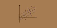
April 21, 2025 - By this I wanted to show you that the parallel lines depend on (w,b) of our hyperplane, if we multiply the equation of hyperplane with a factor greater than 1 then the parallel lines will shrink and if we multiply with a factor less than 1, they expand. We can now say that these lines will move as we do changes in (w,b) and this is how this gets optimized. But what is the optimization function? Let’s calculate it. We know that the aim of SVM is to maximize this margin that means distance (d).
Videos
11:37
SVM algorithm Find Hyperplane Solved Numerical Example in Machine ...
08:27
How to draw a hyper plane in Support Vector Machine | Linear SVM ...
31:55
7.3.2. Math behind Support Vector Machine Classifier - YouTube
05:13
Equation for the Margin (Support Vector Machine) - YouTube
14:00
Support Vector Machine Mathematics Intuition - hyperplane, margin ...
Shuzhan Fan
shuzhanfan.github.io › 2018 › 05 › understanding-mathematics-behind-support-vector-machines
Understanding the mathematics behind Support Vector Machines
May 7, 2018 - SVM works by finding the optimal hyperplane which could best separate the data. The question then comes up as how do we choose the optimal hyperplane and how do we compare the hyperplanes. Let’s first consider the equation of the hyperplane \(w\cdot x + b=0\).
set of methods for supervised statistical learning
Wikipedia
en.wikipedia.org › wiki › Support_vector_machine
Support vector machine - Wikipedia
2 weeks ago - In addition to performing linear classification, SVMs can efficiently perform non-linear classification using the kernel trick, representing the data only through a set of pairwise similarity comparisons between the original data points using a kernel function, which transforms them into coordinates in a higher-dimensional feature space.
scikit-learn
scikit-learn.org › stable › modules › svm.html
1.4. Support Vector Machines — scikit-learn 1.8.0 documentation
Support Vector Machines are powerful tools, but their compute and storage requirements increase rapidly with the number of training vectors. The core of an SVM is a quadratic programming problem (QP), separating support vectors from the rest of the training data.
MIT
web.mit.edu › 6.034 › wwwbob › svm-notes-long-08.pdf pdf
1 An Idiot’s guide to Support vector machines (SVMs) R. Berwick, Village Idiot
Inner products, similarity, and SVMs · 19 · Insight into inner products · Consider that we are trying to maximize the form: LD(ai ) = ai · i=1 · l · ! " 1 · 2 · aia j · i=1 · l · ! yi y j xi #x j · ( ) s.t. ai yi = 0 · i=1 · l · ! & ai $ 0 · The claim is that this function will ...
MathWorks
mathworks.com › statistics and machine learning toolbox › regression › support vector machine regression
Understanding Support Vector Machine Regression - MATLAB & Simulink
Sequential minimal optimization (SMO) is the most popular approach for solving SVM problems [4]. SMO performs a series of two-point optimizations. In each iteration, a working set of two points are chosen based on a selection rule that uses second-order information. Then the Lagrange multipliers for this working set are solved analytically using the approach described in [2] and [1]. ... L for the active set is updated after each iteration. The decomposed equation for the gradient vector is
Mit
ai6034.mit.edu › wiki › images › SVM_and_Boosting.pdf pdf
Useful Equations for solving SVM questions
B. Equations from the boundaries and constraints: ... GHQHUDO IRUP, IRU DQ\ NHUQHO. ... GHQHUDO IRUP, IRU DQ\ NHUQHO. For use when the Kernel is linear. ... ThiV eTXaWiRQ iV XVefXO ZheQ VROYiQg SVM SURbOePV iQ 1D RU 2D, ZheUe Whe ZidWh Rf Whe URad caQ be visuall\ determined.
YouTube
youtube.com › watch
Support Vector Machines (SVM) - the basics | simply explained - YouTube
This video is intended for beginners1. The equation of a straight line2. The general form of a straight line (02:19)3. The distance between a point and a li...
Published August 15, 2022
Analytics Vidhya
analyticsvidhya.com › home › the mathematics behind support vector machine algorithm (svm)
The Mathematics Behind Support Vector Machine Algorithm (SVM)
January 16, 2025 - So, first let’s revise the formulae ... is an equation of a line which will help in segregating the similar categories, and lastly the distance formula between a data point and the line (a boundary separating the categories). Let’s assume we have some data where we (algorithm of SVM) are asked ...
Medium
medium.com › @priyankaparashar54 › support-vector-machine-and-its-mathematical-implementation-c0bdd8b4c699
Support Vector Machine and it’s Mathematical Implementation | by Priyanka Parashar | Medium
June 20, 2020 - The above equation is subjected to the constraint: Then our entire SVM equation boils down to: The hyper parameter ‘c’ defines by what margin we penalize the error. The larger the value of ‘c’ , greater is the chance for the model to become a hard margin classification.


Medium
ankitnitjsr13.medium.com › math-behind-support-vector-machine-svm-5e7376d0ee4d
Math behind SVM (Support Vector Machine) | by MLMath.io | Medium
February 16, 2019 - In first we will formulate SVM optimization problem Mathematically · we will find gradient with respect to learning parameters. we will find the value of parameters which minimizes ||w|| ... The above equation is Primal optimization problem.Lagrange method is required to convert constrained optimization problem into unconstrained optimization problem.
SVM Tutorial
svm-tutorial.com › home › svm - understanding the math - the optimal hyperplane
SVM - Understanding the math : the optimal hyperplane
April 30, 2023 - We now have a unique constraint (equation 8) instead of two (equations 4 and 5) , but they are mathematically equivalent.
ScienceDirect
sciencedirect.com › topics › chemical-engineering › support-vector-machine
Support Vector Machine - an overview | ScienceDirect Topics
Margin (marked as ρ) is the distance between the parallel hyperplanes which are also described by appropriate equations (Fig. 18). The aim of SVM method is to calculate the parameters w and b, so that the distance (ρ) between the parallel hyperplanes separating the data, is maximized.
University of Oxford
robots.ox.ac.uk › ~az › lectures › ml › lect2.pdf pdf
Lecture 2: The SVM classifier
SVM – Optimization · • Learning the SVM can be formulated as an optimization: max · w · 2 · ||w|| subject to w>xi+b ≥1 · if yi = +1 · ≤−1 · if yi = −1 · for i = 1 . . . N · • Or equivalently · min · w ||w||2 · subject to yi · ³ · w>xi + b ·
Medium
medium.com › @tarlanahad › linear-svm-classifier-step-by-step-theoretical-explanation-with-python-implementation-d86c4973dc33
Linear SVM Classifier: Step-by-step Theoretical Explanation with Python Implementation | by Tarlan Ahadli | Medium
August 24, 2021 - The function ‘fit’ is for updating the vector w at each iteration. Function ‘predict’ is for predicting the class of the unknown sample based on the decision rule given in equation 2. Now it’s time to test the performance of SVM class on a linearly separable data [5].
Harvard-iacs
harvard-iacs.github.io › 2018-CS109A › lectures › lecture-20 › presentation › lecture20_svm.pdf pdf
CS109A Introduction to Data Science Pavlos Protopapas and Kevin Rader
Illustration of an SVM · 6 · CS109A, PROTOPAPAS, RADER · Geometry of Decision Boundaries · Recall that the decision boundary is defined by some equation in · terms of the predictors. A linear boundary is defined by: w⊤x + b = 0 (General equation of a hyperplane) Recall that the non-constant ...
Medium
medium.com › analytics-vidhya › basics-of-support-vector-machine-svm-ba6e923dc7b3
Basics of Support Vector Machine (SVM) | by Jinesh Choudhary | Analytics Vidhya | Medium
February 28, 2024 - Now let us move with our first question what is the equation of a line? definitely not a new thing and most of us will reply saying y= mx + b or another form of it is ax+by+c=0 but do you remember if you plot this on paper how will it look like?